京都大学 情報学研究科 知能情報学専攻 2019年8月実施 情報学基礎 F-1

Author

祭音Myyura

Description

Q.1

A hash table is an effective data structure for implementing the operations, e.g. INSERT, SEARCH, and DELETE, in computer systems.

(1.1) What is the advantage of hash tables compared ot directly addressing into an array?

(1.2) Given a hash table of size \(7\) to store integer keys, with linear probing and a hash function \(h(x) = x \text{ mod } 7\), show the content of the hash table after inserting the keys \(0,11,3,7,1,9\) in the given order.

(1.3) Given a hash function \(h\) to hash \(n\) distinct keys into an aray \(T\) of length \(m\) and assuming a uniform hashing, what is the expected cardinality of \(\{\{k, l\}: k \neq l \text{ and } h(k) = h(l)\}\).

Q.2

Breadth first search (BFS) and depth first search (DFS) are two algorithms for traversing trees or graphs.

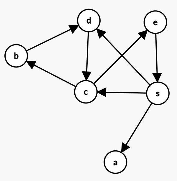
(2.1) Given a set of vertices \(\{a,b,c,d, e,s\}\) of a graph, draw the directed graph according to the folowing vertex adjacency lists:

\[ \begin{aligned} \text{adj}(s) = [a,c,d] \\ \text{adj}(a) = [] \\ \text{adj}(c) = [b,e] \\ \text{adj}(b) = [d] \\ \text{adj}(d) = [c] \\ \text{adj}(e) = [s] \end{aligned} \]

where an adjacency list \(\text{adj}(i)\) denotes the set of neighbors of a vertex \(i\) in the graph, and points to the neighbors of \(i\).

(2.2) Give the visited vertices in an alphabetical order for the graph given in (2.1) using BFS and DFS, respectively. Assume that both algorithms are initially called with the vertex \(s\) and that the vertices are stored in the adjacency lists.

(2.3) Give a recursive algorithm for DFS in a graph.

Kai

Q.1

(1.1)

Operations	Array Time Complexity	Hash Table Time Complexity
Index Access	\(O(1)\)	N/A
Key Access	N/A	\(O(1)\) Average, \(O(n)\) Worst Case
Search	\(O(n)\)	\(O(1)\) Average, \(O(n)\) Worst Case
Insertion	\(O(n)\)	\(O(1)\) Average, \(O(n)\) Worst Case
Deletion	\(O(n)\)	\(O(1)\) Average, \(O(n)\) Worst Case

Compared to array, hash table provides constant time for searching, insertion and deletion operations on average, offers a high-speed data retrieval and manipulation.

(1.2)

(Note: Linear probing is a strategy for resolving collisions, by placing the new key into the closest following empty cell)

[0, 7, 1, 3, 11, 9, ]

(1.3)

Under the assumption of uniform hashing, we will use linearity of expectation to compute this.

Suppose that all the keys are totally ordered \(\{k_1, \dots, k_n\}\). Let \(X_i\) be the number of \(\ell\)'s such that \(\ell > k_i\) and \(h(\ell) = h(k_i)\). So \(X_i\) is the (expected) number of times that key \(k_i\) is collided by those keys hashed afterward. Note that this is the same thing as \(\sum_{j > i} \Pr(h(k_j) = h(k_i)) = \sum_{j > i} 1 / m = (n - i) / m\). Then, by linearity of expectation, the number of collisions is the sum of the number of collisions for each possible smallest element in the collision. The expected number of collisions is

\[ \sum_{i = 1}^n \frac{n - i}{m} = \frac{n^2 - n(n + 1) / 2}{m} = \frac{n^2 - n}{2m}. \]

Q.2

(2.1)

(2.2)

BFS

s, a, c, d, b, e

DFS

s, a, c, b, d, e

(2.3)

DFS(G, u)
    u.visited = true
    for each v ∈ G.adj(u)
        if v.visited == false
            DFS(G, v)

main()
    for each u ∈ G
        u.visited = false
    for each u ∈ G
        DFS(G, u)