東京大学 新領域創成科学研究科 メディカル情報生命専攻 2016年8月実施 問題8 Author zephyr
Description Answer the following questions about linear algebra.
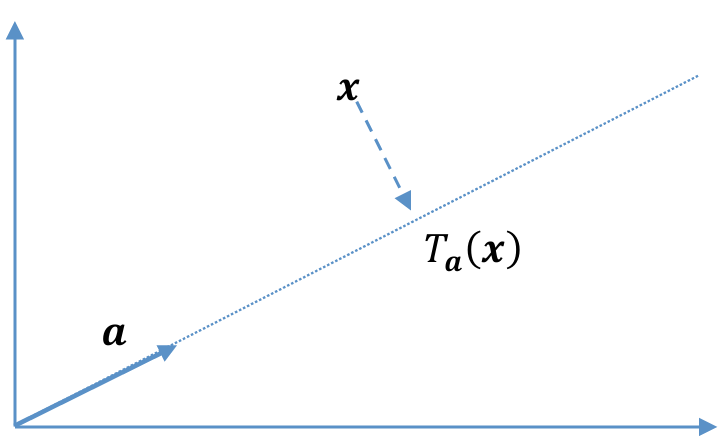
(1) Denote by o \mathbf{o} o a \mathbf{a} a o \mathbf{o} o T a ( x ) T_{\mathbf{a}}(\mathbf{x}) T a ( x ) x \mathbf{x} x a \mathbf{a} a
(1.1) T a ( T a ( x ) ) = T a ( x ) T_{\mathbf{a}}(T_{\mathbf{a}}(\mathbf{x})) = T_{\mathbf{a}}(\mathbf{x}) T a ( T a ( x )) = T a ( x ) x \mathbf{x} x
(1.2) T b ( T a ( x ) ) = o T_{\mathbf{b}}(T_{\mathbf{a}}(\mathbf{x})) = \mathbf{o} T b ( T a ( x )) = o b \mathbf{b} b a \mathbf{a} a
(2) Assume that a real symmetric matrix P \mathbf{P} P P 2 = P \mathbf{P}^2 = \mathbf{P} P 2 = P P \mathbf{P} P
(3) Denote by a 1 , a 2 \mathbf{a_1}, \mathbf{a_2} a 1 , a 2 A = [ a 1 , a 2 ] \mathbf{A} = [\mathbf{a_1}, \mathbf{a_2}] A = [ a 1 , a 2 ]
回答以下有关线性代数的问题。
(1) 用 o \mathbf{o} o a \mathbf{a} a o \mathbf{o} o T a ( x ) T_{\mathbf{a}}(\mathbf{x}) T a ( x ) x \mathbf{x} x a \mathbf{a} a
(1.1) 对于任意二维点 x \mathbf{x} x T a ( T a ( x ) ) = T a ( x ) T_{\mathbf{a}}(T_{\mathbf{a}}(\mathbf{x})) = T_{\mathbf{a}}(\mathbf{x}) T a ( T a ( x )) = T a ( x )
(1.2) 对于任意非零二维向量 b \mathbf{b} b a \mathbf{a} a T b ( T a ( x ) ) = o T_{\mathbf{b}}(T_{\mathbf{a}}(\mathbf{x})) = \mathbf{o} T b ( T a ( x )) = o
(2) 假设一个实对称矩阵 P \mathbf{P} P P 2 = P \mathbf{P}^2 = \mathbf{P} P 2 = P P \mathbf{P} P
(3) 用 a 1 , a 2 \mathbf{a_1}, \mathbf{a_2} a 1 , a 2 A = [ a 1 , a 2 ] \mathbf{A} = [\mathbf{a_1}, \mathbf{a_2}] A = [ a 1 , a 2 ]
题目描述
回答下列线性代数问题:
记零向量为 o \mathbf o o a \mathbf a a T a ( x ) T_{\mathbf a}(\mathbf x) T a ( x ) x \mathbf x x a \mathbf a a
对任意二维点 x \mathbf x x
T a ( T a ( x ) ) = T a ( x ) ; T_{\mathbf a}(T_{\mathbf a}(\mathbf x))=T_{\mathbf a}(\mathbf x); T a ( T a ( x )) = T a ( x ) ;
对任意与 a \mathbf a a b \mathbf b b
T b ( T a ( x ) ) = o . T_{\mathbf b}(T_{\mathbf a}(\mathbf x))=\mathbf o. T b ( T a ( x )) = o .
设实对称矩阵 P \mathbf P P P 2 = P \mathbf P^2=\mathbf P P 2 = P 0 0 0 1 1 1
在三维空间中,列向量 a 1 , a 2 \mathbf a_1,\mathbf a_2 a 1 , a 2
A = [ a 1 , a 2 ] , \mathbf A=[\mathbf a_1,\mathbf a_2], A = [ a 1 , a 2 ] , 用 A \mathbf A A
Kai (1)
(1.1)
The orthogonal projection of x \mathbf{x} x a \mathbf{a} a
T a ( x ) = a ⋅ x a ⋅ a a T_{\mathbf{a}}(\mathbf{x}) = \frac{\mathbf{a} \cdot \mathbf{x}}{\mathbf{a} \cdot \mathbf{a}} \mathbf{a} T a ( x ) = a ⋅ a a ⋅ x a To prove the proposition, we apply T a T_{\mathbf{a}} T a T a ( x ) T_{\mathbf{a}}(\mathbf{x}) T a ( x )
T a ( T a ( x ) ) = T a ( a ⋅ x a ⋅ a a ) T_{\mathbf{a}}(T_{\mathbf{a}}(\mathbf{x})) = T_{\mathbf{a}}\left( \frac{\mathbf{a} \cdot \mathbf{x}}{\mathbf{a} \cdot \mathbf{a}} \mathbf{a} \right) T a ( T a ( x )) = T a ( a ⋅ a a ⋅ x a ) Using the definition of orthogonal projection:
T a ( a ⋅ x a ⋅ a a ) = a ⋅ ( a ⋅ x a ⋅ a a ) a ⋅ a a T_{\mathbf{a}}\left( \frac{\mathbf{a} \cdot \mathbf{x}}{\mathbf{a} \cdot \mathbf{a}} \mathbf{a} \right) = \frac{\mathbf{a} \cdot \left( \frac{\mathbf{a} \cdot \mathbf{x}}{\mathbf{a} \cdot \mathbf{a}} \mathbf{a} \right)}{\mathbf{a} \cdot \mathbf{a}} \mathbf{a} T a ( a ⋅ a a ⋅ x a ) = a ⋅ a a ⋅ ( a ⋅ a a ⋅ x a ) a Simplifying the dot products:
= ( a ⋅ x ) ( a ⋅ a ) ( a ⋅ a ) a ⋅ a a = a ⋅ x a ⋅ a a = \frac{\frac{(\mathbf{a} \cdot \mathbf{x})(\mathbf{a} \cdot \mathbf{a})}{(\mathbf{a} \cdot \mathbf{a})}}{\mathbf{a} \cdot \mathbf{a}} \mathbf{a} = \frac{\mathbf{a} \cdot \mathbf{x}}{\mathbf{a} \cdot \mathbf{a}} \mathbf{a} = a ⋅ a ( a ⋅ a ) ( a ⋅ x ) ( a ⋅ a ) a = a ⋅ a a ⋅ x a Thus:
T a ( T a ( x ) ) = T a ( x ) T_{\mathbf{a}}(T_{\mathbf{a}}(\mathbf{x})) = T_{\mathbf{a}}(\mathbf{x}) T a ( T a ( x )) = T a ( x ) (1.2)
Given b ⋅ a = 0 \mathbf{b} \cdot \mathbf{a} = 0 b ⋅ a = 0
T b ( T a ( x ) ) = T b ( a ⋅ x a ⋅ a a ) T_{\mathbf{b}}(T_{\mathbf{a}}(\mathbf{x})) = T_{\mathbf{b}}\left( \frac{\mathbf{a} \cdot \mathbf{x}}{\mathbf{a} \cdot \mathbf{a}} \mathbf{a} \right) T b ( T a ( x )) = T b ( a ⋅ a a ⋅ x a ) Using the definition of orthogonal projection:
T b ( a ⋅ x a ⋅ a a ) = b ⋅ ( a ⋅ x a ⋅ a a ) b ⋅ b b T_{\mathbf{b}}\left( \frac{\mathbf{a} \cdot \mathbf{x}}{\mathbf{a} \cdot \mathbf{a}} \mathbf{a} \right) = \frac{\mathbf{b} \cdot \left( \frac{\mathbf{a} \cdot \mathbf{x}}{\mathbf{a} \cdot \mathbf{a}} \mathbf{a} \right)}{\mathbf{b} \cdot \mathbf{b}} \mathbf{b} T b ( a ⋅ a a ⋅ x a ) = b ⋅ b b ⋅ ( a ⋅ a a ⋅ x a ) b Since b ⋅ a = 0 \mathbf{b} \cdot \mathbf{a} = 0 b ⋅ a = 0
= ( a ⋅ x ) ( b ⋅ a ) ( a ⋅ a ) b ⋅ b b = ( a ⋅ x ) ⋅ 0 ( a ⋅ a ) ⋅ ( b ⋅ b ) b = 0 = \frac{\frac{(\mathbf{a} \cdot \mathbf{x})(\mathbf{b} \cdot \mathbf{a})}{(\mathbf{a} \cdot \mathbf{a})}}{\mathbf{b} \cdot \mathbf{b}} \mathbf{b} = \frac{(\mathbf{a} \cdot \mathbf{x}) \cdot 0}{(\mathbf{a} \cdot \mathbf{a}) \cdot (\mathbf{b} \cdot \mathbf{b})} \mathbf{b} = 0 = b ⋅ b ( a ⋅ a ) ( a ⋅ x ) ( b ⋅ a ) b = ( a ⋅ a ) ⋅ ( b ⋅ b ) ( a ⋅ x ) ⋅ 0 b = 0 Thus:
T b ( T a ( x ) ) = o T_{\mathbf{b}}(T_{\mathbf{a}}(\mathbf{x})) = \mathbf{o} T b ( T a ( x )) = o (2)
Assume that a real symmetric matrix P \mathbf{P} P P 2 = P \mathbf{P}^2 = \mathbf{P} P 2 = P P \mathbf{P} P
Let P \mathbf{P} P v \mathbf{v} v P \mathbf{P} P λ \lambda λ
P v = λ v \mathbf{P}\mathbf{v} = \lambda \mathbf{v} Pv = λ v Applying P \mathbf{P} P
P 2 v = P ( P v ) = P ( λ v ) = λ P v = λ ( λ v ) = λ 2 v \mathbf{P}^2 \mathbf{v} = \mathbf{P} (\mathbf{P} \mathbf{v}) = \mathbf{P} (\lambda \mathbf{v}) = \lambda \mathbf{P} \mathbf{v} = \lambda (\lambda \mathbf{v}) = \lambda^2 \mathbf{v} P 2 v = P ( Pv ) = P ( λ v ) = λ Pv = λ ( λ v ) = λ 2 v Since P 2 = P \mathbf{P}^2 = \mathbf{P} P 2 = P
P 2 v = P v = λ v \mathbf{P}^2 \mathbf{v} = \mathbf{P} \mathbf{v} = \lambda \mathbf{v} P 2 v = Pv = λ v Thus:
λ 2 v = λ v \lambda^2 \mathbf{v} = \lambda \mathbf{v} λ 2 v = λ v Since v \mathbf{v} v
λ 2 = λ \lambda^2 = \lambda λ 2 = λ Thus, the eigenvalues λ \lambda λ
λ ( λ − 1 ) = 0 \lambda (\lambda - 1) = 0 λ ( λ − 1 ) = 0 Therefore:
λ = 0 or λ = 1 \lambda = 0 \quad \text{or} \quad \lambda = 1 λ = 0 or λ = 1 (3)
Given the matrix A \mathbf{A} A a 1 \mathbf{a_1} a 1 a 2 \mathbf{a_2} a 2 P \mathbf{P} P R 3 \mathbb{R}^3 R 3
Matrix A \mathbf{A} A
A = [ a 1 , a 2 ] \mathbf{A} = [\mathbf{a_1}, \mathbf{a_2}] A = [ a 1 , a 2 ] where A \mathbf{A} A 3 × 2 3 \times 2 3 × 2
Derivation of the Projection Matrix
1. Projection of a Vector
The projection of a vector x \mathbf{x} x A \mathbf{A} A A \mathbf{A} A
P x = c 1 a 1 + c 2 a 2 \mathbf{P}\mathbf{x} = c_1 \mathbf{a_1} + c_2 \mathbf{a_2} Px = c 1 a 1 + c 2 a 2 In matrix form, we write:
P x = A c \mathbf{P}\mathbf{x} = \mathbf{A}\mathbf{c} Px = Ac where c \mathbf{c} c
c = [ c 1 c 2 ] \mathbf{c} = \begin{bmatrix}
c_1 \\
c_2
\end{bmatrix} c = [ c 1 c 2 ] 2. Finding the Coefficients
To determine the coefficients c \mathbf{c} c
A T ( x − A c ) = 0 \mathbf{A}^T (\mathbf{x} - \mathbf{A}\mathbf{c}) = \mathbf{0} A T ( x − Ac ) = 0 This equation implies:
A T x = A T A c \mathbf{A}^T \mathbf{x} = \mathbf{A}^T \mathbf{A} \mathbf{c} A T x = A T Ac The columns of A \mathbf A A ∥ A c ∥ 2 > 0 \|\mathbf A\mathbf c\|^2>0 ∥ Ac ∥ 2 > 0 c \mathbf c c A T A \mathbf A^T\mathbf A A T A
c = ( A T A ) − 1 A T x \mathbf{c} = (\mathbf{A}^T \mathbf{A})^{-1} \mathbf{A}^T \mathbf{x} c = ( A T A ) − 1 A T x 3. Constructing the Projection Matrix
Substituting c \mathbf{c} c
P x = A ( A T A ) − 1 A T x \mathbf{P}\mathbf{x} = \mathbf{A} (\mathbf{A}^T \mathbf{A})^{-1} \mathbf{A}^T \mathbf{x} Px = A ( A T A ) − 1 A T x Since this holds for any vector x \mathbf{x} x P \mathbf{P} P
P = A ( A T A ) − 1 A T \mathbf{P} = \mathbf{A} (\mathbf{A}^T \mathbf{A})^{-1} \mathbf{A}^T P = A ( A T A ) − 1 A T Knowledge 对称矩阵 特征值和特征向量 投影矩阵
重点词汇
Orthogonal projection 正交投影
Symmetric matrix 对称矩阵
Eigenvalue 特征值
Column vector 列向量
Subspace 子空间
Projection matrix 投影矩阵
参考资料
Gilbert Strang, "Linear Algebra and Its Applications," Chap. 3, 5.
David C. Lay, "Linear Algebra and Its Applications," Chap. 6.
Reference