東京大学 情報理工学系研究科 創造情報学専攻 2024年8月実施 筆記試験 第1問

标签：

• Tokyo-University
• Markov-Chain
• Matrix-Limit

Author

祭音Myyura (with the help of an anonymous contributor), itsuitsuki

Description

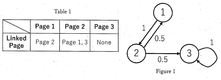
Suppose that there are $N$ web pages. A user staying at a web page at time $t$ ($t \ge 0$) will move to one of the linked pages at time $t+1$ with equal probability. If there are no linked pages, the user will stay at the same page as time $t$. Let $p_n^{(t)}$ ($1 \le n \le N$) denote the probability of the user staying at the $n$-th page at time $t$, and $\boldsymbol{p}^{(t)} = (p_1^{(t)} \ p_2^{(t)} \dots p_N^{(t)})^\mathrm{T}$ denote the vector that summarizes them.

First, let us consider the case of $N = 3$ shown in Table 1. When there are three web pages shown in Table 1, the state transition diagram that represents a user's state is depicted as a graph in Figure 1. Each node in the graph shown in Figure 1 corresponds one-to-one to a page in Table 1, and an edge represents a transition between the pages from time $t$ to time $t+1$. The value appended to an edge shows the probability of the transition occurring. Note that when there are no linked pages and a user keeps staying at the same page, it is interpreted as a transition to the same page as time $t$.

Answer the following questions.

(1) Given $\boldsymbol{p}^{(0)} = (1 \ 0 \ 0)^\mathrm{T}$, find $\boldsymbol{p}^{(1)}$ and $\boldsymbol{p}^{(2)}$.

(2) Represent $\boldsymbol{p}_1^{(t)}$ and $\boldsymbol{p}_2^{(t)}$ using $t$. $\boldsymbol{p}^{(0)}$ is the same as in Question (1).

(3) Find $\boldsymbol{p}^{(t)}$ when $t \to \infty$. $\boldsymbol{p}^{(0)}$ is the same as in Question (1).

Next, we introduce an operation called "jump" that occurs during a move between pages from time $t$ to time $t + 1$ with a constant probability $\alpha > 0$. When a jump occurs, the user moves to one of $N$ pages (including the current page) with equal probability. When a jump does not occur, the user moves to one of the linked pages with equal probability in the same manner as before (if there are no linked pages, the user will keep staying at the current page).

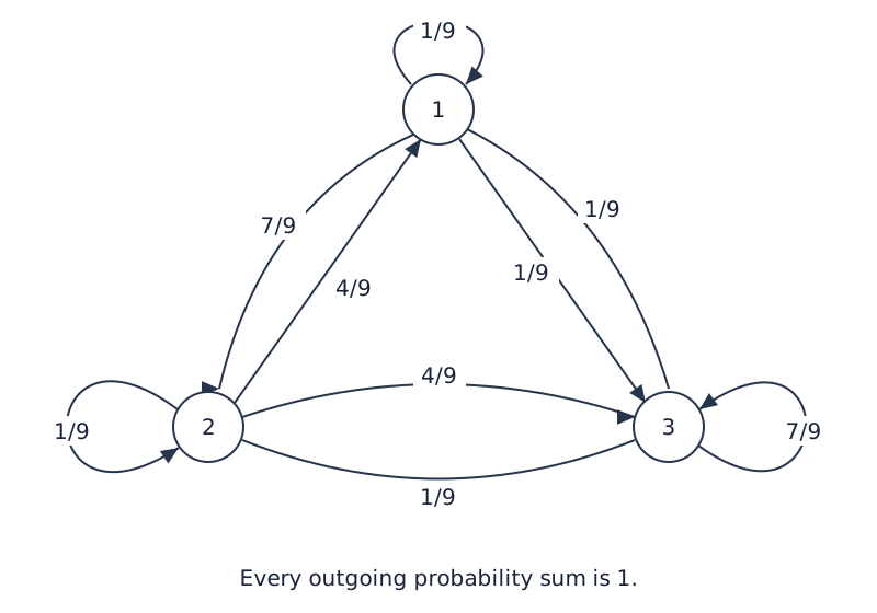
(4) We introduce the jump operation into the case in Table 1. Suppose that $\alpha = 1/3$. Draw a state transition diagram for this case. Also, find the transition probability matrix $A$ that satisfies the following equation

$$\boldsymbol{p}^{(t+1)} = A\boldsymbol{p}^{(t)}.$$

(5) When $\boldsymbol{p}^{(t+1)} = \boldsymbol{p}^{(t)} (= \boldsymbol{p})$, this $\boldsymbol{p}$ is called a stationary distribution. Find the stationary distribution in the case of Question (4).

Finally, we consider the transition probability matrix $R$ and stationary distribution of a general case where the jump operation is introduced. For answering the following questions, you can use the Perron–Frobenius theorem described below.

Perron–Frobenius theorem for positive matrices

A positive square matrix has a positive eigenvalue $k$ that satisfies the following. Here, a positive matrix is a matrix whose elements are all positive real numbers.

(i) For the absolute value of an arbitrary eigenvalue $\lambda$ other than $k$, $|\lambda| < k$ holds.

(ii) The eigenvalue $k$ is a simple root (i.e., has the multiplicity of 1), and there exists a positive eigenvector that belongs to the eigenvalue $k$. Here, a positive vector is a vector whose elements are all positive real numbers.

(iii) There are no positive eigenvectors that belong to eigenvalues other than $k$.

(6) Show that $R^\mathrm{T}$, the transpose of $R$, has 1 as an eigenvalue, and that this is the eigenvalue with the largest absolute value.

(7) Show that a stationary distribution exists uniquely. Here, you can assume the following fact as given; In general, a square matrix and its transpose have the same set of eigenvalues.

(8) Show that, by iteratively computing $\boldsymbol{p}^{(t)}$ following the equation $\boldsymbol{p}^{(t+1)} = R\boldsymbol{p}^{(t)}$, regardless of the initial probability distribution $\boldsymbol{p}^{(0)}$, $\boldsymbol{p}^{(t)}$ converges to the stationary distribution when $t \to \infty$. You can assume that $\boldsymbol{p}^{(0)}$ can be represented as a linear combination of eigenvectors, $\boldsymbol{p}^{(0)} = \sum_{i=1}^N c_i \boldsymbol{x}_i$. Here, $\boldsymbol{x}_i$ denotes the $i$-th eigenvalue of $R$ while $c_i$ is its coefficient.

题目描述

有 $N$ 个网页。用户在时刻 $t\ge0$ 位于某页，时刻 $t+1$ 等概率移动到该页链接的某个网页；若该页无外链，则留在原页。记位于第 $n$ 页的概率为 $p_n^{(t)}$，并令

$$\boldsymbol p^{(t)}=(p_1^{(t)},p_2^{(t)},\ldots,p_N^{(t)})^\mathsf T.$$

先考虑原文表 1 的 $N=3$ 情形，图 1 给出状态转移图，边标号为转移概率；无外链时停留也视为自环转移。

1. 给定 $\boldsymbol p^{(0)}=(1,0,0)^\mathsf T$，求 $\boldsymbol p^{(1)},\boldsymbol p^{(2)}$。
2. 在相同初始分布下，用 $t$ 表示 $p_1^{(t)},p_2^{(t)}$。
3. 求 $t\to\infty$ 时的 $\boldsymbol p^{(t)}$。

再引入“跳转”：每次从 $t$ 到 $t+1$ 以固定概率 $\alpha>0$ 跳到 $N$ 页中的任意一页（包括当前页），各页等概率；不跳转时仍按原链接等概率移动，无外链则停留。

4. 对表 1 情形取 $\alpha=1/3$，画新状态转移图，并求满足

   $$\boldsymbol p^{(t+1)}=A\boldsymbol p^{(t)}$$

   的转移矩阵 $A$。

5. 若 $\boldsymbol p^{(t+1)}=\boldsymbol p^{(t)}=\boldsymbol p$，称 $\boldsymbol p$ 为平稳分布。求第 4 问的平稳分布。

最后考虑一般含跳转操作的转移矩阵 $R$。可使用正矩阵的 Perron–Frobenius 定理：正方阵所有元素均为正时，存在正特征值 $k$，且

1. 其他任意特征值 $\lambda$ 均满足 $|\lambda|<k$；

2. $k$ 是单根，并有属于 $k$ 的正特征向量；

3. 其他特征值没有正特征向量。

4. 证明 $R^\mathsf T$ 有特征值 1，且 1 是绝对值最大的特征值。

5. 证明平稳分布存在且唯一。可使用“一般方阵与其转置具有相同特征值集合”。

6. 证明无论初始概率分布 $\boldsymbol p^{(0)}$ 为何，按

   $$\boldsymbol p^{(t+1)}=R\boldsymbol p^{(t)}$$

   迭代时，$t\to\infty$ 都收敛到平稳分布。可假定初始向量能写成 $R$ 的特征向量线性组合 $\boldsymbol p^{(0)}=\sum_{i=1}^Nc_i\boldsymbol x_i$。

Kai

(1)

$$p^{(1)}=(0,1,0)^{T}, \ p^{(2)}=(0.5,0,0.5)^{T}$$

(2)

Let $M$ denote the transition matrix. Then we have

$$M = \begin{pmatrix} 0 & 0.5 & 0 \\ 1 & 0 & 0 \\ 0 & 0.5 & 1 \end{pmatrix}$$

and

$$p^{(1)} = M p^{(0)}, \ p^{(2)} = M p^{(1)} = M^{2} p^{(0)}$$

Since $p_1^{(t+1)}=\frac12p_2^{(t)}$ and $p_2^{(t+1)}=p_1^{(t)}$,

$$p_1^{(t)}= \begin{cases}2^{-t/2},&t\text{ even},\\0,&t\text{ odd},\end{cases} \qquad p_2^{(t)}= \begin{cases}0,&t\text{ even},\\2^{-(t-1)/2},&t\text{ odd}.\end{cases}$$

(3)

The eigenvalues of $M$ are

$$\det(\lambda I - M) = (\lambda - 1)(\lambda^2 - 0.5) = 0$$

$$\Rightarrow \lambda_1 = 1, \ \lambda_2 = \frac{\sqrt{2}}{2}, \ \lambda_3 = -\frac{\sqrt{2}}{2}$$

and the corresponding eigenvectors are

$$v_1 = (0,0,1)^{\top}, \ v_2 = (1-\sqrt{2}, -2+\sqrt{2}, 1)^{\top}, \ v_3=(1+\sqrt{2}, -2-\sqrt{2}, 1)^{\top}$$

Hence we have

$$\begin{aligned} \lim_{t \to \infty} p^{(t)} &= \lim_{t \to \infty} M^t p^{(0)} \\ &= \lim_{t \to \infty} \{c_1 \cdot 1^t \cdot v_1 + c_2 \left(\frac{1}{\sqrt{2}}\right)^t v_2 + c_3 \left(-\frac{1}{\sqrt{2}}\right)^t v_3 \} \\ &= c_1 v_1 \\ &= (0,0,1)^{\top} \quad \text{(since $p^{t}$ is a probability distribution)} \end{aligned}$$

(4)

When $\alpha = \frac{1}{3}$,

• If no jump occurs, the transition is $M$.
• If a jump occurs, each destination has probability $1/3$.

$$\begin{aligned} A &= (1-\alpha)M + \alpha \begin{bmatrix} 1/3 & 1/3 & 1/3 \\ 1/3 & 1/3 & 1/3 \\ 1/3 & 1/3 & 1/3 \end{bmatrix} \\ &= \frac{2}{3} \begin{bmatrix} 0 & 0.5 & 0 \\ 1 & 0 & 0 \\ 0 & 0.5 & 1 \end{bmatrix} + \frac{1}{3} \begin{bmatrix} 1/3 & 1/3 & 1/3 \\ 1/3 & 1/3 & 1/3 \\ 1/3 & 1/3 & 1/3 \end{bmatrix} \\ &= \begin{bmatrix} 0 & 3/9 & 0 \\ 6/9 & 0 & 0 \\ 0 & 3/9 & 6/9 \end{bmatrix} + \begin{bmatrix} 1/9 & 1/9 & 1/9 \\ 1/9 & 1/9 & 1/9 \\ 1/9 & 1/9 & 1/9 \end{bmatrix} \\ &= \frac{1}{9} \begin{bmatrix} 1 & 4 & 1 \\ 7 & 1 & 1 \\ 1 & 4 & 7 \end{bmatrix} \end{aligned}$$

Thus the diagram has outgoing probabilities $1\to(1,2,3):(1,7,1)/9$, $2\to(1,2,3):(4,1,4)/9$, and $3\to(1,2,3):(1,1,7)/9$.

(5)

Let $p = (x, y, z)^{\top}$. Then, by solving $Ap = p$, i.e., the following equations

$$\begin{cases} 9x = x + 4y + z \\ 9y = 7x + y + z \\ 9z = x + 4y + 7z \\ x + y + z = 1 \end{cases}$$

we have

$$p = \frac{1}{21} (4, 5, 12)^{\top}$$

(6)

Since $R$ is a transition probability matrix, we have

$$\sum_{i} R_{ij} = 1 \quad \forall j$$

hence

$$R^{\top} \boldsymbol{1} = 1 \cdot \boldsymbol{1}$$

which implies that $1$ is an eigenvalue of $R^{\top}$.

Since $R^{\top}$ is positive and $\boldsymbol 1$ is a positive eigenvector, the Perron--Frobenius eigenvalue is $1$. Therefore every other eigenvalue has absolute value less than $1$.

(7)

Since $R$ and $R^{\top}$ have the same eigenvalues, $R$ has eigenvalue $1$. Perron--Frobenius gives a positive eigenvector $v$; normalizing it by $p=v/(\boldsymbol1^{\top}v)$ yields a stationary distribution $Rp=p$.

For uniqueness, assume that there exist two different stationary distributions $p$ and $q$.

Then by definition we have

$$Rp = 1 \cdot p, \quad Rq = 1 \cdot q$$

i.e., $p$ and $q$ are both eigenvectors corresponding to the eigenvalue $\lambda=1$.

(the Perron Frobenius theorem) Since for positive matrices, $1$ is a simple root, which means that the eigenspace for $\lambda=1$ is 1-dimensional. Hence

$$p = cq$$

Note that $p$ and $q$ are both probability distributions, i.e., $\sum p_i = \sum q_j = 1$. Thus $c = 1$, which is contradictory to the assumption that $p$ and $q$ are different.

Therefore the stationary distribution is unique.

(8)

Expand the initial state $p^{(0)}$ in the eigenbasis of $R$:

$$p^{(0)} = c_1 x_1 + \sum_{i=2}^{N} c_i x_i,$$

where $x_1$ is the eigenvector associated with the eigenvalue $\lambda_1 = 1$, and each $x_i$ corresponds to $\lambda_i$.

Apply the matrix $R$ for $t$ steps:

$$p^{(t)} = R^t p^{(0)} = c_1 (1)^t x_1 + \sum_{i=2}^{N} c_i (\lambda_i)^t x_i.$$

By the Perron–Frobenius theorem, for all $i \ge 2$ we have $|\lambda_i| < 1$. Hence $\lim_{t \to \infty} (\lambda_i)^t = 0$, and therefore

$$\lim_{t \to \infty} p^{(t)} = c_1 x_1.$$

Now left-multiply both sides by $\boldsymbol{1}^T$ (the row vector of all ones, i.e., summing all components). Since total probability is conserved, $\boldsymbol{1}^T p^{(t)} = 1$ for all $t$. Thus,

$$1 = \boldsymbol{1}^T (c_1 x_1) = c_1(\boldsymbol{1}^T x_1).$$

Assuming $x_1$ is normalized so that its entries sum to $1$, we have $\boldsymbol{1}^T x_1 = 1$, which implies $c_1 = 1$. Therefore,

$$\lim_{t \to \infty} p^{(t)} = x_1,$$

i.e., the distribution converges to the unique stationary distribution.