東京大学 情報理工学系研究科 創造情報学専攻 2017年8月実施 筆記試験 第1問

标签：

• Tokyo-University
• Decision-Tree
• Decision-Tree-Pruning

Author

tomfluff, 祭音Myyura, itsuitsuki

Description

A data set $S$ including eight data is given as in Figure 1. Each datum is in the form of $(x_1, x_2, x_3, x_4, y) \in \{0, 1\}^5$. Below we consider how to construct a rule from $S$ for classifying $\boldsymbol{x} = (x_1, x_2, x_3, x_4)$ into $y = 1$ or $y = 0$. Answer the following questions.

Figure 1: Data set

$t$	$x_1$	$x_2$	$x_3$	$x_4$	$y$
1	1	0	0	1	1
2	1	1	0	0	1
3	1	0	1	1	1
4	0	1	1	0	1
5	0	0	1	1	0
6	0	0	1	0	0
7	0	0	0	1	0
8	1	1	1	0	0

(1) Let us consider the code-length required for encoding a binary string $z = z_1, \dots, z_n$ of length $n$ ($z_i \in \{0, 1\}, i = 1, \dots, n$). In general, for a finite set $G$, the code-length required for encoding one element $g \in G$ is given by $\log |G|$ (bit), where the logarithm is to the base 2. Show that, for a binary string $z$ of length $n$ in which the number of occurrences of $1$ is $k$, the code-length required for encoding $z$ and $k$ itself is at most:

$$\begin{align} \log(n + 1) + \log \ _nC_k \text{ (bit),} \tag{1} \end{align}$$

where the value of the number $n$ is given in advance and the code-length can be non-integer valued.

Below the value of Eq.(1) for $z$ is denoted as $L(z)$.

(2) Let the probability of $y = 1$ for a datum with $x_1 = 1$ be $\theta$. Then calculate the least squares estimate of $\theta$ from Figure 1. The least squares estimate of $\theta$ is the value of $\theta$ that minimizes $\sum_{t:x_1=1} (y(t) - \theta)^2$ where $y(t)$ denotes the value of $y$ for the $t$-th datum and $\sum_{t:x_1=1}$ denotes the sum taken over all the data such that $x_1 = 1$.

(3) Let $y$ be a binary string obtained by concatenating the values of $y$ for all the data in $S$ in Figure 1. Let $y^{(i)}_1$ be a binary string obtained by concatenating the values of $y$ for all the data in $S$ such that $x_i = 1$ and let $y^{(i)}_0$ be a binary string obtained by concatenating the values of $y$ for all the data in $S$ such that $x_i = 0$ ($i = 1, 2, 3, 4$). For example, the indexes of data in $S$ such that $x_1 = 1$ are $1$, $2$, $3$, $8$, so the binary string obtained by concatenating the values of $y$ corresponding to them is $y^{(1)}_1 = 1110$. We define the measure of goodness of classifying data by partitioning $S$ based on whether $x_i = 1$ or $x_i = 0$ as follows:

$$\begin{align} \Delta(i|y) \overset{\text{def}}{=} L(y^{(i)}_1) + L(y^{(i)}_0) \quad (i = 1, 2, 3, 4). \tag{2} \end{align}$$

We consider that the smaller the value of Eq.(2) is, the more the value of $x_i$ contributes to the classification of $y$. Find $i$ that minimizes $\Delta(i|y)$. Hereinafter, when there are more than one $x_i$’s that minimize the value of Eq.(2), one is chosen randomly from among them.

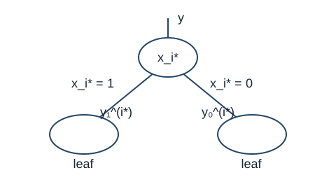
(4) Let the value of $i$ obtained in Question (3) be $i^*$. $S$ is partitioned into two sets according to whether $x_{i^*} = 1$ or $x_{i^*} = 0$, then $y$ is also partitioned into two strings: $y^{(i^*)}_1$ and $y^{(i^*)}_0$. It can be represented using a tree structure as shown in Figure 2. We call it a partitioning tree. We call $y^{(i^*)}_1$ and $y^{(i^*)}_0$ partitioned strings. We further partition each of $y^{(i^*)}_1$ and $y^{(i^*)}_0$, by finding $i \ (\neq i^*)$ minimizing $\Delta(i|y^{(i^*)}_1)$ and minimizing $\Delta(i|y^{(i^*)}_0)$, respectively. Let this partitioning of a leaf be repeated until the following stopping rule is fulfilled: The depth of a leaf (the number of partitionings from the root to the leaf) is two, or the partitioned string arriving at a leaf is all $y = 1$ or all $y = 0$. Find the partitioning tree that is finally obtained.

(5) For the resulting partitioning tree, for a partitioned string arriving at each leaf, we assign $y = 1$ to the leaf if the number of occurrences of $y = 1$ in this string is larger than that of $y = 0$, and assign $y = 0$ to the leaf if the number of occurrences of $y = 1$ is smaller than that of $y = 0$. When the number of occurrences of $y = 1$ is the same as that of $y = 0$, we assign randomly $y = 1$ or $y = 0$ to the leaf. This tree can be used for predicting the value of $y$ for any new datum. That is, when $(x_1, x_2, x_3, x_4)$ in the new datum is given
and arrives at a leaf, the tree predicts the value of its corresponding $y$ as the value of $y$ assigned to the leaf. Here, even if we change the stopping rule in Question (4) to construct a larger tree from a training data set $S$ so that the values of $y$ for data reaching at each leaf are all $y = 1$ or all $y = 0$, such a tree doesn’t necessarily predict the value of $y$ for a new datum with higher accuracy. Explain the reason.

(6) Consider a general case where for a positive integer $d \geq 2$, a set $S$ of multi-dimensional data in the form of $(x_1, \dots, x_d, y) \in \{0, 1\}^{d+1}$ and a partitioning tree $\mathcal{T}$ are given. Let $\mathcal{M}$ be a set of all subtrees which share the root of $\mathcal{T}$ and are obtained by pruning $\mathcal{T}$ starting
from its leaves. We define the following penalized criterion for evaluating the goodness of a subtree $M \in \mathcal{M}$ for the given $S$:

$$\begin{align} N_L(M) C_L + N_I(M) C_I + \sum_u L(y_u), \tag{3} \end{align}$$

where $N_L(M)$ is the total number of leaves in $M$ and $N_I(M)$ is the total number of inner nodes in $M$. $C_L$ and $C_I$ are given positive constants. The sum in the third term in Eq.(3) is taken over all the leaves $\{u\}$ in $M$ and $y_u$ is the binary string obtained by concatenating the values of $y$ for all the data which reach the leaf $u$. The smaller the value of Eq.(3) is, the better $M$ is. Give an algorithm that finds $M$ minimizing the criterion Eq.(3) from $\mathcal{M}$ and $S$, and runs as efficiently as possible in computation time.

Kai

(1) - By Myyura

The notation $_nC_k$ usually represents "n choose k".

For a fixed $n$ and $k$, the total number of possible binary strings that satisfy these conditions is given by the binomial coefficient $\binom{n}{k}$, i.e. $_nC_k$.

To uniquely identify any of these strings, we need a code of length:

$$\log \binom{n}{k}$$

The length $n$ should be included as part of the encoded message, hence the total encoding length is:

$$\log(n + 1) + \log \binom{n}{k} \text{ (bit),} \tag{1}$$

(2) - By tomfluff

Let us fine a $\theta$ such that the least squares is minimized. Let us denote least squares as $f(\theta )$.

$$f(\theta )=\sum_{t:x_1=1}(y(t) - \theta )^2$$

$$f(\theta )=(1 - \theta )^2+(1 - \theta )^2+(1 - \theta )^2+(0 - \theta )^2$$

$$f(\theta )=3(1 - \theta )^2+(- \theta )^2$$

$$f'(\theta )=-6+6\theta +2\theta = 0$$

$$\Rightarrow 8\theta = 6 \Rightarrow \theta=\frac{3}{4}$$

Therefore, when $\theta = \frac{3}{4}$ the least squares function is minimized.

(3) - By itsuitsuki

• $\Delta(1|y)=4+2\log 5$
• $\Delta(2|y)=4+\log 5+2\log 3$
• $\Delta(3|y)=4+\log 5+2\log 3$
• $\Delta(4|y)=2+2\log 5+2\log 3$ Hence $i=1$ minimizes $\Delta(i|y)$.

(4) - By tomfluff

Note: Any mistakes here are derived from the issues with (1) mentioned before.

(5)

In machine learning there are the concepts of bias and variance. The bias indicates how much the generated prediction function fits the relationships between the data and the prediction. And variance indicates how much the prediction function fits "new" data (testing data). When the prediction function fits the training data too well it is called "over fitting" and over fitting leads to low bias but high variance. In the mentioned case, extending the tree would result in over fitting the prediction function to the data set. Meaning that on new data the variance will be large and it will not improve the overall prediction.

(6) - by Gemini

The algorithm will work as Cost-Complexity Pruning. Tomfluff (the previous solution provider in this problem) misrecognizes this as a Minimum Error Pruning technique which is different. Similar pruning algorithms include PEP (Pessimistic Error Pruning), etc.

The algorithm is dynamic programming:

1. Post-order traverse every node;
2. For each internal node $u$, we can choose to
   1. Prune the node into a leaf with contribution to criterion $\text{Cost}_{\text{prune}}(u) = C_L + L(\text{all data under }u)$
   2. Keep the subtree rooted at $u$ with contribution $\text{Cost}{\text{keep}}(u) = C_I + \sum{v\in \text{children}(u)} \text{Cost}_{\min}(u)
3. Choose a minimum-contribution action with $\text{Cost}_{\min}(u) = \min(\text{Cost}_{\text{prune}}(u), \text{Cost}_{\text{keep}}(u))$. When pruning, mark this subtree rooted at $u$ as a leaf.

Since in this DP, all nodes are traversed and computed for at once, the time complexity is $O(|\mathcal T|)$.