東京大学 情報理工学系研究科 創造情報学専攻 2013年8月実施 筆記試験 第3問

标签：

• Tokyo-University
• Image-Filtering-and-Moments
• K-Nearest-Neighbors
• Nearest-Centroid-Classifier
• Graphics

Author

itsuitsuki

Description

Official examination, archived Japanese PDF. We consider the problem of distinguishing between two hand-written alphabets "C" and "I" using image processing and pattern recognition techniques. Figure 1 shows an input image X. Let $i$ and $j$ denote integers corresponding to the $x$ and $y$ coordinates of a pixel. The value of a pixel $(i, j)$ is represented by $f(i, j)$. Here, we take the top-left pixel as the origin $(0, 0)$ of the coordinates.

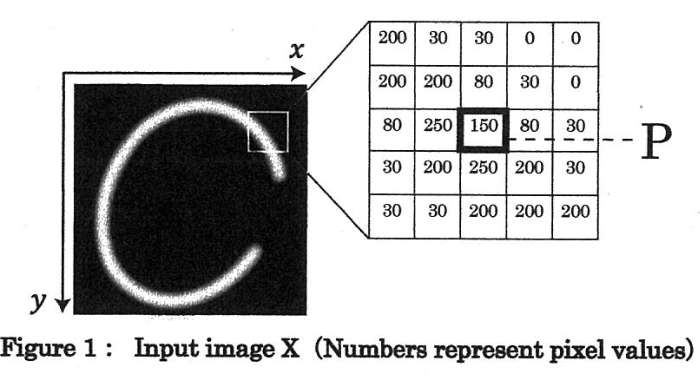
Following the procedure below, we extract some features to quantify the properties of the input image. First, we apply a $3 \times 3$ size linear filter. Let $g(i, j)$ denote the output value of the filter for a pixel $(i, j)$, which is defined as $g(i, j) = \sum_{n=-1}^{1} \sum_{m=-1}^{1} f(i+m, j+n)h(m, n),$ where $h(m, n)$ is the array that contains the coefficients of the filter ($m$ and $n$ are integer values). Answer the following questions.

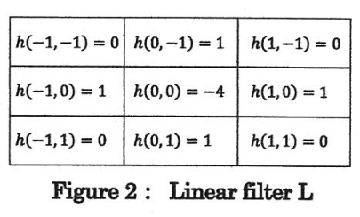
(1) We apply the linear filter L illustrated in Figure 2 to the image X. Compute the output value for the pixel P in Figure 1.

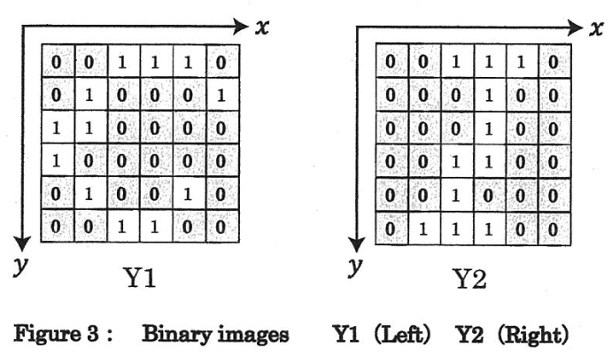
Next, we reduce the resolution of the filtered image to $6 \times 6$ pixels and binarize its values. Specifically, the converted image is represented as $f(i, j) = \{0, 1\} (0 \le i, j \le 5)$. Figure 3 shows two examples of binary images Y1 and Y2. We extract features called "image moments" from them. The image moment of order $(p + q)$ is defined as $M_{pq} = \sum_{i, j} i^p j^q f(i, j)$. For example, we can see that $M_{00}$ corresponds to the [ (A) ] of the figure in the binary image, and $(M_{10}/M_{00}, M_{01}/M_{00})$ corresponds to its [ (B) ].

(2) Fill in the blanks (A) and (B) with appropriate words. Also, compute the image moments $M_{00}$ and $M_{10}$ of Y1 and Y2 respectively.

Taking a pair of two features $(M_{00}, M_{10})$ extracted by the above procedure as an input pattern, we classify this into one of two classes ("C" or "I"). Table 1 lists the values of features of four "C" and four "I" training examples. Also, Figure 4 shows their plots on a two-dimensional graph.

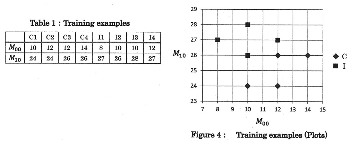
(3) We classify an input pattern using the $k$ nearest neighbor ($k$-NN) method. Namely, a pattern is classified into the class that has the largest number of samples among its $k$ nearest training examples. Suppose we have a new pattern of an input image with the features $(M_{00}, M_{10}) = (13, 27)$. Classify this pattern into "C" or "I" using the $k$-NN method and describe the reason when $k=1$ and $k=3$, respectively. Distance between any two patterns is defined in terms of the Euclidean distance.

(4) As an alternative classification algorithm, we classify an input pattern into the class where the mean of its training examples is nearest to the pattern in terms of the Euclidean distance. Show the equation that defines the boundary of discrimination, and the methodology of discrimination using it. Also, classify the pattern $(M_{00}, M_{10}) = (13, 27)$ using the methodology.

(5) Compare the two algorithms described at (3) and (4) and discuss their advantages respectively.

题目描述

用图像处理和模式识别区分手写字母 “C” 与 “I”。图 1 为输入图像 $X$。像素横、纵坐标分别为整数 $i,j$，像素值为 $f(i,j)$，左上角像素为原点 $(0,0)$。

首先使用 $3\times3$ 线性滤波器提取特征。像素 $(i,j)$ 的输出为

$$g(i,j)=\sum_{n=-1}^{1}\sum_{m=-1}^{1}f(i+m,j+n)h(m,n),$$

其中 $h(m,n)$ 为滤波器系数阵列。

1. 将图 2 的线性滤波器 $L$ 作用于图像 $X$，计算图 1 中像素 $P$ 的输出值。

2. 把滤波后图像降采样为 $6\times6$ 并二值化，使 $f(i,j)\in\{0,1\}$（$0\le i,j\le5$）。图 3 给出二值图像 Y1、Y2。定义 $(p+q)$ 阶图像矩

   $$M_{pq}=\sum_{i,j}i^pj^qf(i,j).$$

   填写：$M_{00}$ 对应图形的【A】，而

   $$\left(\frac{M_{10}}{M_{00}},\frac{M_{01}}{M_{00}}\right)$$

   对应图形的【B】；并分别计算 Y1、Y2 的 $M_{00}$ 与 $M_{10}$。

3. 取特征对 $(M_{00},M_{10})$ 作为输入模式，分类为 C 或 I。原文表 1、图 4 给出四个 C 与四个 I 训练样本的特征。对新样本 $(13,27)$，分别用 $k=1$ 和 $k=3$ 的 $k$ 近邻法分类并说明理由；距离采用欧氏距离，类别由 $k$ 个最近训练样本中的多数决定。

4. 另一方法把样本分到“训练样本均值离它最近”的类别。写出判别边界方程及用它分类的方法，并判定 $(13,27)$ 的类别。

5. 比较第 3、4 问两种分类算法，分别讨论其优点。

题中像素值、滤波器系数、二值图和训练数据沿用原文图表。

Kai

(1) Filter output

The filter is the four-neighbor discrete Laplacian: center coefficient $-4$, horizontal/vertical neighbors $1$, and diagonal neighbors $0$. At $P$ the center is 150 and the upper, left, right and lower neighbors are 80, 250, 80 and 250. Hence

$$\boxed{g(P)=80+250+80+250-4\cdot150=60.}$$

No image-boundary convention is needed because all required pixels are supplied.

(2) Image moments

(A) is area (the number of foreground pixels), and (B) is the centroid or center of mass of uniform foreground pixels. The centroid requires $M_{00}>0$.

For checking the sums, the two binary arrays from Figure 3 are, with row index $j$ increasing downward and column index $i$ increasing to the right:

$$Y_1=\begin{pmatrix} 0&0&1&1&1&0\\ 0&1&0&0&0&1\\ 1&1&0&0&0&0\\ 1&0&0&0&0&0\\ 0&1&0&0&1&0\\ 0&0&1&1&0&0 \end{pmatrix},\qquad Y_2=\begin{pmatrix} 0&0&1&1&1&0\\ 0&0&0&1&0&0\\ 0&0&0&1&0&0\\ 0&0&1&1&0&0\\ 0&0&1&0&0&0\\ 0&1&1&1&0&0 \end{pmatrix}.$$

For $Y_1$, the row foreground counts are $(3,2,2,1,2,2)$ and the row sums of horizontal coordinates are $(9,6,1,0,5,5)$. For $Y_2$, these are $(3,1,1,2,1,3)$ and $(9,3,3,5,2,6)$. Therefore

$$\boxed{Y_1:\ M_{00}=12,\ M_{10}=26;\qquad Y_2:\ M_{00}=11,\ M_{10}=28.}$$

$M_{10}$ weights the horizontal coordinate $i$, not the vertical coordinate $j$.

(3) Nearest neighbors

The numerical data in Table 1 and squared distances from $(13,27)$ are:

Sample	$M_{00}$	$M_{10}$	Squared distance
C1	10	24	18
C2	12	24	10
C3	12	26	2
C4	14	26	2
I1	8	27	25
I2	10	26	10
I3	10	28	10
I4	12	27	1

For $k=1$, the unique nearest example is I4, so the class is $\boxed{\mathrm I}$. For $k=3$, the neighbors are I4, C3 and C4. Two of these three are C, so the class is $\boxed{\mathrm C}$. The tie between C3 and C4 does not create a tie at the third-neighbor boundary because both are included.

(4) Nearest class mean

The class means are

$$\boldsymbol\mu_C=(12,25),\qquad \boldsymbol\mu_I=(10,27).$$

Write the input as $(u,v)=(M_{00},M_{10})$. The boundary is the perpendicular bisector of the two means:

$$(u-12)^2+(v-25)^2=(u-10)^2+(v-27)^2,$$

or

$$\boxed{v=u+15.}$$

The difference “squared distance to C minus squared distance to I” is $4(v-u-15)$. Thus classify as C when $v<u+15$, and as I when $v>u+15$, with an explicit arbitrary tie rule on the line. At $(13,27)$ the squared distances are 5 and 9, respectively, so the decision is $\boxed{\mathrm C}$.

(5) Comparison

The $k$-NN method retains individual examples and can represent nonlinear or multimodal class shapes without restricting each class to one center. Choosing $k>1$ reduces sensitivity to an isolated mislabeled point, but the result depends on $k$, sampling density, feature scaling and distance. A naive query costs $O(nd)$ for distances to $n$ examples in $d$ dimensions, plus neighbor selection, and needs the training examples in memory.

Nearest-mean classification stores only one $d$-dimensional mean per class and compares a query to those means, so prediction is cheaper and the model is compact. Averaging also smooths sample noise when one center summarizes each class well. However, a single mean can lie between separated clusters and ignores their shapes and spreads; with Euclidean distance its pairwise boundaries are linear. Both methods here use the raw features and the specified Euclidean metric; rescaling the moments would define a different classifier.