東京大学 情報理工学系研究科 創造情報学専攻 2013年8月実施 筆記試験 第1問

标签：

• Tokyo-University
• Online-Learning-with-Expert-Advice
• Regret-Bound

Author

itsuitsuki

Description

Official examination, archived Japanese PDF. We consider a weather prediction system in which a single senior predictor predicts a weather probability distribution on the basis of $N$ predictors' prediction results. Below the system is described in details. There are $N$ weather predictors, each of whom outputs a weather probability distribution once a day. Here the weather is a binary random variable taking a value 1 or 0 only (1 means "fine" while 0 means "not fine"). It is assumed that the weather is independent of a day. Let the probability distribution that the $i$-th predictor outputs on the $t$-th day be $P_i^{(t)}(X)$ ($X \in \{1, 0\}$) where we let $0 < P_i^{(t)}(X) < 1$ ($X \in \{1, 0\}$). There is a senior predictor who aggregates the outputs of the $N$ predictors. On the $t$-th day, the senior predictor takes a weighted average over the probability distributions output by the $N$ predictors to output a weather probability distribution $\hat{P}^{(t)}(X)$ ($X \in \{1, 0\}$). Here the weight on the $i$-th predictor on the $t$-th day is denoted as $v_i^{(t)}$ ($\sum_{i=1}^N v_i^{(t)} = 1, v_i(t) > 0$ ($i = 1, \dots, N$)). That is, on the $t$-th day, $\hat{P}^{(t)}(X)$ is given by $\sum_{i=1}^N v_i^{(t)} P_i^{(t)}(X)$ (see Figure 1). On the $t$-th day, after the senior predictor ouputs, the real outcome $x_t \in \{1, 0\}$ of the weather on the day is reported. This process goes on sequentially with respect to $t$. In the above setting, answer the following questions.

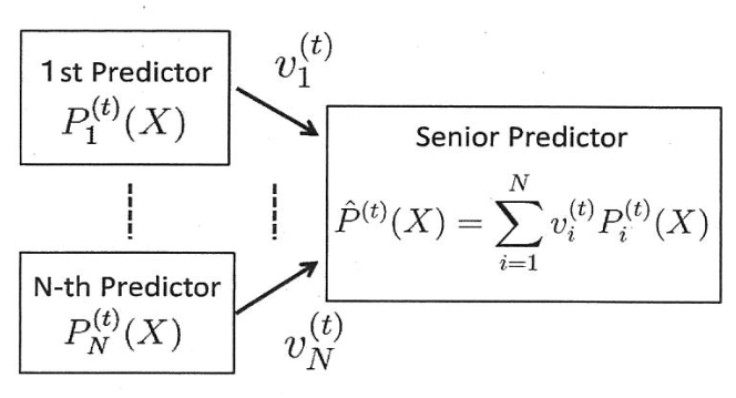
(1) Assume that the senior predictor defines the weight $v_i^{(t)}$ of the $i$-th predictor on the $t$-th day so that the ratio of $v_i^{(t)}$s with respect to $i$ is equal to that of their corresponding likelihoods with respect to the sequence of the past $t-1$ data: $x^{t-1} = x_1 \dots x_{t-1}$. That is, when we denote the likelihood of the $i$-th predictor with respect to $x^{t-1}$ as $w_i^{(t-1)}$,

the following equation holds: For each $t$, $v_1^{(t)} : \dots : v_N^{(t)} = w_1^{(t-1)} : \dots : w_N^{(t-1)}.$ The likelihood of the $i$-th predictor with respect to $x^{t-1}$ is calculated as $w_i^{(t-1)} = \prod_{j=1}^{t-1} P_i^{(j)}(X = x_j)$, where we denote $P_i^{(j)}(X = x_j)$ as $P_i^{(j)}(x_j)$ and we set $P_i^{(0)}(x_0) = 1$ ($i = 1, \dots, N$). In this setting, for each $i$, show a relation between $w_i^{(t)}$ and $w_i^{(t-1)}$, and derive a formula for calculating $v_i^{(t+1)}$ using $w_i^{(t-1)}$ and $P_i^{(t)}(x_t)$ ($i = 1, \dots, N$).

(2) Suppose that the senior predictor predicts the weather probability distribution sequentially with respect to $t$ for $T$ days. Then under the setting of $v_i^{(t)}$ as in (1), write an algorithm for the senior predictor to output a weather probability distribution and update the weights for predictors every day, and show the order of its computation time in terms of $N$ and $T$. Here the initial weight for each predictor is set as follows: $v_1^{(0)} = \dots = v_N^{(0)} = 1/N.$

(3) When the prediction is sequentially made for $T$ days, we define the cumulative predictive loss for the senior predictor with respect to the sequence $x^T = x_1 \dots x_T$ of observed real coutcome as follows: $Loss(x^T) = \sum_{t=1}^T \left( -\log \hat{P}^{(t)}(x_t) \right).$ Then write $Loss(x^T)$ as a function of $P_i^{(t)}(x_t)$ ($i = 1, \dots, N, t = 1, \dots, T$) and $N$. Here the logarithm is the natural logarithm.

(4) Prove that the senior predictor's cumulative loss for $T$ days defined in (3) is at most $\log N$ larger than the least cumulative loss over all $i$-th predictors for $T$ days. Here the cumulative loss for the $i$-th predictor for $T$ days is defined as $\sum_{t=1}^T (-\log P_i^{(t)}(x_t))$ ($i = 1, \dots, N$).

题目描述

考虑一个在线天气预测系统：$N$ 名预测者每天各输出一次二元天气 $X\in\{1,0\}$ 的概率分布，其中 1 表示晴、0 表示非晴，且假定不同日期的天气相互独立。第 $i$ 名预测者在第 $t$ 天输出 $P_i^{(t)}(X)$，对两个取值均有 $0<P_i^{(t)}(X)<1$。

一名高级预测者汇总这 $N$ 个结果。第 $t$ 天给第 $i$ 人的权重为 $v_i^{(t)}>0$，且 $\sum_{i=1}^Nv_i^{(t)}=1$，输出加权混合分布

$$\hat P^{(t)}(X)=\sum_{i=1}^Nv_i^{(t)}P_i^{(t)}(X).$$

高级预测者输出后，才公布当天真实结果 $x_t\in\{1,0\}$，上述过程随 $t$ 依次进行。

1. 权重之比等于各预测者对过去 $t-1$ 天结果序列 $x^{t-1}=x_1\cdots x_{t-1}$ 的似然之比：

   $$v_1^{(t)}:\cdots:v_N^{(t)} =w_1^{(t-1)}:\cdots:w_N^{(t-1)},$$

   其中

   $$w_i^{(t-1)}=\prod_{j=1}^{t-1}P_i^{(j)}(X=x_j),$$

   简记 $P_i^{(j)}(X=x_j)$ 为 $P_i^{(j)}(x_j)$，并令 $P_i^{(0)}(x_0)=1$。对每个 $i$，写出 $w_i^{(t)}$ 与 $w_i^{(t-1)}$ 的关系，并推导用 $w_i^{(t-1)}$ 和 $P_i^{(t)}(x_t)$ 计算 $v_i^{(t+1)}$ 的公式。

2. 连续预测 $T$ 天，按第 1 问的权重规则写出高级预测者每天输出混合概率并更新各预测者权重的算法，分析关于 $N,T$ 的时间复杂度。初始权重均为

   $$v_1^{(0)}=\cdots=v_N^{(0)}=\frac1N.$$

3. 对真实序列 $x^T=x_1\cdots x_T$，定义高级预测者的累计对数损失

   $$Loss(x^T)=\sum_{t=1}^T-\log\hat P^{(t)}(x_t).$$

   用所有 $P_i^{(t)}(x_t)$（$i=1,\ldots,N;\ t=1,\ldots,T$）及 $N$ 表示 $Loss(x^T)$，其中 $\log$ 为自然对数。

4. 第 $i$ 名预测者的 $T$ 日累计损失为

   $$\sum_{t=1}^T-\log P_i^{(t)}(x_t).$$

   证明高级预测者的累计损失至多比所有单个预测者中最小的累计损失多 $\log N$。

Kai

(1) Likelihood and weight updates

The empty-product likelihood is $w_i^{(0)}=1$. Multiplying by the newly observed outcome probability gives

$$\boxed{w_i^{(t)}=w_i^{(t-1)}P_i^{(t)}(x_t).}$$

Weights proportional to the likelihoods must be normalized to sum to one. Thus

$$\boxed{v_i^{(t+1)}= \frac{w_i^{(t-1)}P_i^{(t)}(x_t)} {\sum_{j=1}^Nw_j^{(t-1)}P_j^{(t)}(x_t)} =\frac{v_i^{(t)}P_i^{(t)}(x_t)}{\hat P^{(t)}(x_t)}.}$$

All denominators are positive by the stipulated strictly positive probabilities.

(2) Sequential algorithm

Use the uniform weights for the first day's prediction. The statement calls the initial vector $v^{(0)}$; in the day-based notation of part (1), this is $v^{(1)}$, since it precedes any observation. It is the same uniform initialization, not an extra update using future data.

v[i] = 1/N for i = 1,...,N
for t = 1,...,T:
    obtain today's N predictive distributions P[i]
    prediction[0] = sum(v[i] * P[i][0] for i = 1,...,N)
    prediction[1] = sum(v[i] * P[i][1] for i = 1,...,N)
    output prediction
    observe the actual outcome x[t]
    z = prediction[x[t]]
    for i = 1,...,N:
        v[i] = v[i] * P[i][x[t]] / z

The senior predictor takes $\boxed{O(NT)}$ arithmetic operations and $O(N)$ working storage, excluding the predictors' own computation and stored output history. It outputs before observing that day's outcome. For long sequences, store log-likelihoods and normalize using log-sum-exp to avoid numerical underflow from products of many small probabilities; this retains the same asymptotic arithmetic count.

(3) Cumulative loss

Write $W_t=\sum_i w_i^{(t)}$, so $W_0=N$. Then

$$\hat P^{(t)}(x_t)= \frac{\sum_iw_i^{(t-1)}P_i^{(t)}(x_t)}{W_{t-1}} =\frac{W_t}{W_{t-1}}.$$

Multiplying over days telescopes:

$$\prod_{t=1}^T\hat P^{(t)}(x_t)=\frac{W_T}{W_0} =\frac1N\sum_{i=1}^N\prod_{t=1}^TP_i^{(t)}(x_t).$$

Consequently

$$\boxed{Loss(x^T)=-\log\left(\frac1N\sum_{i=1}^N \prod_{t=1}^TP_i^{(t)}(x_t)\right).}$$

The uniform average is outside the products: this mixture selects one expert for the whole sequence in its likelihood representation, rather than selecting a fresh uniform expert each day.

(4) Bound relative to the best expert

Let $L_i=-\sum_t\log P_i^{(t)}(x_t)$ and choose $i_*\in\arg\min_iL_i$. Since each likelihood is nonnegative,

$$\frac1N\sum_i e^{-L_i}\ge\frac1N e^{-L_{i_*}}.$$

Applying the decreasing function $-\log$ gives

$$\boxed{Loss(x^T)\le L_{i_*}+\log N=\min_i L_i+\log N.}$$

This is a bound for every realized sequence, not merely for an expected loss. Indeed the algebraic proof itself does not require stochastic independence of the daily outcomes. At $N=1$ the two losses coincide; for $N>1$ and finite $T$, strict positivity makes the displayed upper bound strict, although it can be approached arbitrarily closely.