東京大学 情報理工学系研究科 創造情報学専攻 2009年8月実施 筆記試験 第1問

标签：

• Tokyo-University
• Shortest-Path-Problem

Author

itsuitsuki

Description

出典：大学公式問題冊子の保存版。 Given a directed graph $G = (V, E)$, we would like to find all-pairs shortest path lengths which are the all shortest path lengths between every pair of vertices, where the size of the set $V, |V| = n$. Let $e_{uv}$ denote a directed edge from a vertex $u$ to a vertex $v$, and $\delta_{uv}$ denote the length of the edge $e_{uv}$. The graph $G$ may have a negative length edge but does not have any negative length cycle. The length of the edge from the vertex $u$ to the same vertex $u, \delta_{uu} = 0$, and when there exists no edge from the vertex $u$ to the vertex $v$, $\delta_{uv} = \infty$.

Algorithm 1 on the next page outputs the single-source shortest path lengths. Let $s \in V$ be a single source vertex, the shortest path length from the vertex $s$ to a vertex $v \in V$ is stored in $d(v)$. Algorithm 2 outputs the all-pairs shortest path lengths table $D$, where the length of the shortest path from a vertex $u$ to a vertex $v$ is stored in $D(u, v)$. Each algorithm uses $d^{(k)}$ and $D^{(k)} (k = 0, 1, \dots)$ to store interim results, respectively. Answer the following questions.

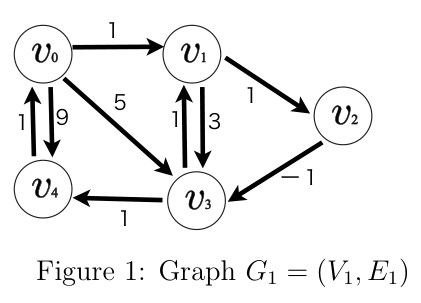
(1) Apply Algorithm 1 to the graph $G_1 = (V_1, E_1)$ in Figure 1 to obtain the shortest path length from a single-source vertex $v_0$. Table 1 shows $d^{(0)}$ in Algorithm 1. Show the single-source path length $d^{(1)}, d^{(2)}, d^{(3)}$, and $d^{(4)}$ from the single-source vertex $v_0$.

(2) Apply Algorithm 2 to the graph $G_1 = (V_1, E_1)$ in Figure 1 to obtain the all-pairs shortest path lengths. Table 2 shows $D^{(0)}$ in Algorithm 2. Show the selected vertex $w \in V_1$ in the Main Loop and the corresponding table $D^{(1)}, D^{(2)}, D^{(3)}, D^{(4)}$, and $D^{(5)}$.

(3) To obtain all-pairs shortest path lengths, consider Algorithm 1-ALL which applies Algorithm 1 for all vertices in $V$ as a single-source vertex. Compare Algorithm 1-ALL and Algorithm 2.

Table 1: $d^{(0)}$ in Algorithm 1

destination
$v_0$	0
$v_1$	$\infty$
$v_2$	$\infty$
$v_3$	$\infty$
$v_4$	$\infty$

Table 2: $D^{(0)}$ in Algorithm 2

source\destination	$v_0$	$v_1$	$v_2$	$v_3$	$v_4$
$v_0$	0	1	$\infty$	5	9
$v_1$	$\infty$	0	1	3	$\infty$
$v_2$	$\infty$	$\infty$	0	-1	$\infty$
$v_3$	$\infty$	1	$\infty$	0	1
$v_4$	1	$\infty$	$\infty$	$\infty$	0

Algorithm definitions — independent English summary

This is an independent summary of the algorithm definitions.

Algorithm 1: initialize $d^{(0)}(s)=0$ and $d^{(0)}(v)=\infty$ for $v\ne s$, and perform $n-1$ rounds of edge relaxation. The printed assignment for each edge $e_{uv}$ is

$d^{(k)}(v)=\min\{d^{(k-1)}(v),\ d^{(k-1)}(u)+\delta_{uv}\}.$

For the shortest-path calculation below, initialize $d^{(k)}\gets d^{(k-1)}$, and for each edge accumulate

$d^{(k)}(v)\gets\min\{d^{(k)}(v),\ d^{(k-1)}(u)+\delta_{uv}\}.$

The answer below uses this accumulating relaxation.

Algorithm 2: initialize $D^{(0)}(u,v)=\delta_{uv}$. Select each vertex $w$ once, and use the preceding matrix to form

$D^{(k+1)}(u,v)=\min\{D^{(k)}(u,v),\ D^{(k)}(u,w)+D^{(k)}(w,v)\}$

for all $u,v$, then increment $k$. The order of the selected vertices must be stated when giving intermediate matrices.

题目描述

给定含 $n=|V|$ 个顶点的有向图 $G=(V,E)$，求任意两顶点之间的最短路径长度。用 $e_{uv}$ 表示从 $u$ 到 $v$ 的有向边，$\delta_{uv}$ 表示其长度。图中允许负权边，但不存在负权环；约定 $\delta_{uu}=0$，若 $u$ 到 $v$ 无边，则 $\delta_{uv}=\infty$。

原文所给算法 1 求单源最短路：源点为 $s\in V$，$d(v)$ 存储 $s$ 到 $v$ 的最短距离，并用 $d^{(k)}$ 存储中间结果。算法 2 求全源最短路矩阵 $D$，其中 $D(u,v)$ 存储 $u$ 到 $v$ 的最短距离，并用 $D^{(k)}$ 存储中间结果。

1. 对图 1 的 $G_1=(V_1,E_1)$，以 $v_0$ 为源点执行算法 1。初值表为

   终点	$d^{(0)}$
   $v_0$	$0$
   $v_1$	$\infty$
   $v_2$	$\infty$
   $v_3$	$\infty$
   $v_4$	$\infty$

   写出 $d^{(1)},d^{(2)},d^{(3)},d^{(4)}$。

2. 对同一图执行算法 2。初始矩阵为

   源点 \ 终点	$v_0$	$v_1$	$v_2$	$v_3$	$v_4$
   $v_0$	$0$	$1$	$\infty$	$5$	$9$
   $v_1$	$\infty$	$0$	$1$	$3$	$\infty$
   $v_2$	$\infty$	$\infty$	$0$	$-1$	$\infty$
   $v_3$	$\infty$	$1$	$\infty$	$0$	$1$
   $v_4$	$1$	$\infty$	$\infty$	$\infty$	$0$

   写出主循环各轮选中的 $w\in V_1$，以及相应的 $D^{(1)},D^{(2)},D^{(3)},D^{(4)},D^{(5)}$。

3. 定义算法 1-ALL：把 $V$ 中每个顶点依次作为源点运行算法 1，以得到全源最短路。比较算法 1-ALL 与算法 2。

Kai

(1)

上記の補足どおり、同じラウンド内の各入辺の候補を累積して最小値を取るBellman–Ford法として計算する。$d^{(k)}(v)$ は高々 $k$ 本の辺を使って到達する最短距離である。

$k$	$v_0$	$v_1$	$v_2$	$v_3$	$v_4$
0	0	$\infty$	$\infty$	$\infty$	$\infty$
1	0	1	$\infty$	5	9
2	0	1	2	4	6
3	0	1	2	1	5
4	0	1	2	1	2

例えば $v_3$ への距離は $v_0\to v_1\to v_2\to v_3$ により $1+1-1=1$、$v_4$ へはさらに長さ1の辺を使って2となる。負閉路がないため最短路には単純路を選べ、必要な辺数は高々 $n-1=4$ 本である。

(2)

$w=v_0,v_1,v_2,v_3,v_4$ の順で選ぶ。各行・列は $v_0,\ldots,v_4$ の順である。

$$D^{(1)}=\begin{pmatrix} 0&1&\infty&5&9\\ \infty&0&1&3&\infty\\ \infty&\infty&0&-1&\infty\\ \infty&1&\infty&0&1\\ 1&2&\infty&6&0 \end{pmatrix},\qquad(w=v_0)$$

$$D^{(2)}=\begin{pmatrix} 0&1&2&4&9\\ \infty&0&1&3&\infty\\ \infty&\infty&0&-1&\infty\\ \infty&1&2&0&1\\ 1&2&3&5&0 \end{pmatrix},\qquad(w=v_1)$$

$$D^{(3)}=\begin{pmatrix} 0&1&2&1&9\\ \infty&0&1&0&\infty\\ \infty&\infty&0&-1&\infty\\ \infty&1&2&0&1\\ 1&2&3&2&0 \end{pmatrix},\qquad(w=v_2)$$

$$D^{(4)}=\begin{pmatrix} 0&1&2&1&2\\ \infty&0&1&0&1\\ \infty&0&0&-1&0\\ \infty&1&2&0&1\\ 1&2&3&2&0 \end{pmatrix},\qquad(w=v_3)$$

$$\boxed{D^{(5)}=\begin{pmatrix} 0&1&2&1&2\\ 2&0&1&0&1\\ 1&0&0&-1&0\\ 2&1&2&0&1\\ 1&2&3&2&0 \end{pmatrix}},\qquad(w=v_4)$$

各段では、新しく許された中継点 $w$ を通らない経路と、$u\to w\to v$ と分けられる経路の最小値を比較する。全頂点を許した $D^{(5)}$ が全点対最短距離である。

(3)

Algorithm 1は修正済みBellman–Ford法、Algorithm 2はFloyd–Warshall法として比較する。どちらも負辺を扱えるが、ここでは負閉路がないことを使っている。

Algorithm 1は1始点につき $n-1$ ラウンドで全 $|E|$ 辺を調べる。各ラウンドの長さ $n$ の初期化も数えると $O(n(n+|E|))$、全始点なら $O(n^2(n+|E|))$ である。通常の $|E|\ge n$ の範囲では、それぞれ $O(n|E|)$、$O(n^2|E|)$ と書ける。Algorithm 2は中継点と始終点の三重ループにより $O(n^3)$。

従って $|E|=\Theta(n^2)$ の密なグラフでは、全始点Bellman–Fordの $O(n^4)$ に対してFloyd–Warshallが $O(n^3)$ で有利である。$|E|=\Theta(n)$ の疎なグラフでは両者とも $O(n^3)$ だが、前者は辺リストを直接利用できる。作業領域はBellman–Fordが2本の距離ベクトルで $O(n)$、Floyd–Warshallが行列を再利用して $O(n^2)$。全点対の結果自体を保存するなら、いずれも $O(n^2)$ の出力領域が必要となる。