京都大学 情報学研究科 知能情報学専攻 2023年8月実施 専門科目 S-5

标签：

• Kyoto-University
• Fourier-Slice-Theorem
• Discrete-Fourier-Transform
• Fast-Fourier-Transform
• Sampling-Theorem-and-Aliasing
• Fourier-Analysis

Author

祭音Myyura

Description

設問1

2次元信号 $f(x, y)$ の2次元フーリエ変換を

$$F(u, v) = \iint_{-\infty}^{\infty} f(x, y) e^{-j(ux+vy)} dxdy$$

とする。ただし $j$ は虚数単位である。 また $f(x, y)$ のある軸 $l$ への投影を、軸 $l$ 上の各点における、$l$ に垂直な直線に沿った $f(x, y)$ の線積分とする。以下の問いに答えよ。

(1) $f(x, y)$ を $x$ 軸に投影した信号 $p(x)$ の1次元フーリエ変換を、$F(u, v)$ を用いて表せ。

(2) 原点を中心として $x$ 軸を反時計回りに角度 $\theta$ 回転して得られた $s$ 軸上に $f(x, y)$ を投影した信号を $p_\theta(s)$ とする。 $p_\theta(s)$ の $s$ についての1次元フーリエ変換を $F(u, v)$ を用いて表せ。

設問2

長さ $N$ の離散時間信号 $x[n]$ の $N$ 点離散フーリエ変換 $X[k]$ を

$$X[k] = \sum_{n=0}^{N-1} x[n] W_N^{kn}, \quad W_N = e^{-j\frac{2\pi}{N}}$$

とする。ただし $j$ は虚数単位、$n, k = 0, \ldots, N-1$ であり、$N$ は正の偶数とする。以下の問いに答えよ。

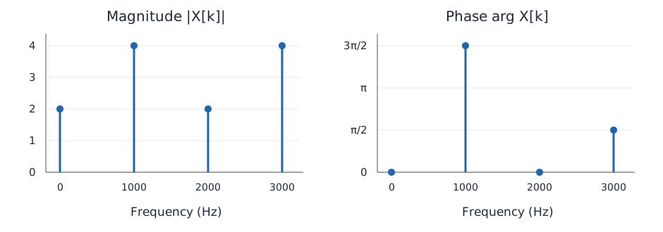
(1) 観測系列 $x_0[n] = \{x_0[0], x_0[1], x_0[2], x_0[3]\} = \{1, 2, 1, -2\}$ を、ある信号を 4000Hz で等間隔にサンプリングすることで得たとする。 $x_0[n]$ の４点離散フーリエ変換を計算し、周波数（Hz）に対応する振幅スペクトルおよび位相スペクトルを図示せよ。

(2) ２つの要素数 $N$ の実数値系列 $x_1[n]$ および $x_2[n]$ の $N$ 点離散フーリエ変換を、１回の $N$ 点離散フーリエによって計算する方法を導出せよ。

(3) 要素数 $2N$ の実数値系列の $2N$ 点離散フーリエ変換を、１回の $N$ 点離散フーリエ変換によって計算する方法を導出せよ。

Kai

設問1

(1)

By the definition of projection, we have

$$p(x) = \int_{-\infty}^{\infty}f(x,y)dy$$

hence the 1D Fourier transform of $p(x)$ is

$$\int_{-\infty}^{\infty}\left(\int_{-\infty}^{\infty}f(x,y)dy\right)e^{-jux}dx = \int_{-\infty}^{\infty}\int_{-\infty}^{\infty}f(x,y)e^{-j(ux+0\cdot y)}dxdy = F(u, 0)$$

(2)

Let $(s,t)$ denote the coordinates obtained by rotating $(x, y)$ counterclockwise by an angle $\theta$. Then we have

$$\begin{pmatrix} s\\ t \end{pmatrix} = \begin{pmatrix} \cos\theta&-\sin\theta\\ \sin\theta&\cos\theta \end{pmatrix} \begin{pmatrix} x\\ y \end{pmatrix} \Rightarrow \begin{cases} x = s\cos\theta-t\sin\theta\\ y = s\sin\theta+t\cos\theta \end{cases}$$

by calculating the Jacobian determinant

$$J = \begin{vmatrix} \cos\theta&-\sin\theta\\ \sin\theta&\cos\theta \end{vmatrix} = \cos^{2}\theta+\sin^{2}\theta = 1$$

we know that $f(x,y)dxdy{=}f(s,t)dsdt$. Hence the 1D Fourier transform of $p_{\theta}(x)$ is

$$\begin{aligned} \int_{-\infty}^{\infty}\left(\int_{-\infty}^{\infty}f(s,t)dt\right)e^{-jus}ds &= \int_{-\infty}^{\infty}\int_{-\infty}^{\infty}f(s,t)e^{-j(us+0\cdot t)}dsdt\\ &= \int_{-\infty}^{\infty}\int_{-\infty}^{\infty}f(x,y)e^{-j(u\cos\theta x+(-u\sin\theta)y)}dxdy\\ &= F(u\cos\theta, -u\sin\theta) \end{aligned}$$

設問2

(1)

The 4-point discrete Fourier transform of $x_0[n]$:

$$\begin{pmatrix} X[0]\\ X[1]\\ X[2]\\ X[3] \end{pmatrix} = \begin{pmatrix} W_{4}^{0}&W_{4}^{0}&W_{4}^{0}&W_{4}^{0}\\ W_{4}^{0}&W_{4}^{1}&W_{4}^{2}&W_{4}^{3}\\ W_{4}^{0}&W_{4}^{2}&W_{4}^{4}&W_{4}^{6}\\ W_{4}^{0}&W_{4}^{3}&W_{4}^{6}&W_{4}^{9} \end{pmatrix} \begin{pmatrix} x[0]\\ x[1]\\ x[2]\\ x[3] \end{pmatrix} = \begin{pmatrix} 1&1&1&1\\ 1&-j&-1&j\\ 1&-1&1&-1\\ 1&j&-1&-j \end{pmatrix} \begin{pmatrix} 1\\ 2\\ 1\\ -2 \end{pmatrix} = \begin{pmatrix} 2\\ -4j\\ 2\\ 4j \end{pmatrix}$$

Fig. magnitude and phase spectra

(2)

$$\begin{aligned} X[k] &= \sum_{n=0}^{N-1}x[n]W_{N}^{kn}\\ &= \sum_{n=0}^{N-1}x[n]\cos\left(2\pi-\frac{2\pi kn}{N}\right) + j\sum_{n=0}^{N-1}x[n]\sin\left(2\pi-\frac{2\pi kn}{N}\right)\\ &= \sum_{n=0}^{N-1}x[n]\cos\frac{2\pi n(N-k)}{N} + j\sum_{n=0}^{N-1}x[n]\sin\frac{2\pi n(N-k)}{N}\\ &= \text{Re } X[N-k]-j\text{Im } X[N-k] \end{aligned}$$

which implies that

$$\begin{align} \begin{cases} \text{Re } X[k] = \text{Re } X[N-k]\\ \text{Im } X[k] = -\text{Im } X[N-k] \end{cases} \tag{j} \end{align}$$

Let $y[n] = x_{1}[n]+j x_{2}[n]$. Let $X_{1}[k],X_{2}[k],Y[k]$ denote the discrete Fourier transform of $x_{1}[n],x_{2}[n],y_{n}$, respectively. Then,

$$\begin{align} Y[k] &= \sum_{n=0}^{N-1}(x_{1}[n]+j x_{2}[n])W_{N}^{kn} \nonumber \\ &= \sum_{n=0}^{N-1}x_{1}[n]W_{N}^{kn}+j\sum_{n=0}^{N-1}x_{2}[n]W_{N}^{kn} \nonumber \\ &= X_{1}[k]+iX_{2}[k] \nonumber \\ &= (\text{Re } X_{1}[k]+j\text{Im } X_{1}[k])+j(\text{Re } X_{2}[k]+j \text{Im } X_{2}[k]) \nonumber \\ &= (\text{Re } X_{1}[k]-\text{Im } X_{2}[k])+j(\text{Im } X_{1}[k]+\text{Re } X_{2}[k]) \tag{ii} \end{align}$$

By (i) we know that

$$\begin{align} Y[N-k] &= (\text{Re } X_{1}[N-k]-\text{Im } X_{2}[N-k])+j(\text{Im } X_{1}[N-k]+\text{Re } X_{2}[N-k]) \nonumber \\ &= (\text{Re } X_{1}[k]+\text{Im } X_{2}[k])+j(-\text{Im } X_{1}[k]+\text{Re } X_{2}[k]) \tag{iii} \end{align}$$

and by (ii), (iii) we have

$$\begin{align} \begin{cases} \displaystyle X_{1}[k] = \frac{\text{Re } Y[k]+\text{Re } Y[N-k]}{2}+j\frac{\text{Im } Y[k]-\text{Im } Y[N-k]}{2}\\ \displaystyle X_{2}[k] = \frac{\text{Im } Y[k]+\text{Im } Y[N-k]}{2}-j\frac{\text{Re } Y[k]-\text{Re } Y[N-k]}{2} \end{cases} \tag{iv} \end{align}$$

(3)

By definition we know that $W_{N}^{2kn}{=}W_{N/2}^{kn}$ and $W_{N}^{kN}{=}1$, hence we have

$$\begin{aligned} X[2k] &= \sum_{n=0}^{N-1}x[n]W_{2N}^{2kn}+\sum_{n=N}^{2N-1}x[n]W_{2N}^{2kn}\\ &= \sum_{n=0}^{N-1}x[n]W_{2N}^{2kn}+\sum_{n=0}^{N-1}x[n+N]W_{2N}^{2k(n+N)}\\ &= \sum_{n=0}^{N-1}x[n]W_{N}^{kn}+\sum_{n=0}^{N-1}x[n+N]W_{N}^{k(n+N)}\\ &= \sum_{n=0}^{N-1}x[n]W_{N}^{kn}+\sum_{n=0}^{N-1}x[n+N]W_{N}^{kn}\\ &= \sum_{n=0}^{N-1}(x[n]+x[n+N])W_{N}^{kn}\\ \end{aligned}$$

Similarly, since $W_{2N}^{N}{=}{-}1$, we have

$$\begin{aligned} X[2k+1] &= \sum_{n=0}^{N-1}x[n]W_{2N}^{(2k+1)n}+\sum_{n=0}^{N-1}x[n+N]W_{2N}^{(2k+1)(n+N)}\\ &= \sum_{n=0}^{N-1}\left(x[n]+x[n+N]W_{2N}^{(2k+1)N}\right)W_{2N}^{(2k+1)n}\\ &= \sum_{n=0}^{N-1}\left(x[n]+x[n+N]W_{2N}^{N}\right)W_{2N}^{2kn}W_{2N}^{n}\\ &= \sum_{n=0}^{N-1}\left(x[n]-x[n+N]\right)W_{2N}^{n}W_{N}^{kn} \end{aligned}$$

Therefore, let $y[n]{=}x[n]{+}x[n+N]$ and $z[n]{=}x[n]{-}x[n+N]$, we have

$$\begin{aligned} \begin{cases} X[2k] = \sum_{n=0}^{N-1}y[n]W_{N}^{kn}\\ X[2k] = \sum_{n=0}^{N-1}y[n]W_{2N}^{n}W_{N}^{kn} \end{cases} \end{aligned}$$

which implies that $2N$-point discrete Fourier transforms can be obtained using two executions of the $N$-point Fourier transform.

By using the result from the previous question (2), it has been demonstrated that the $N$-point discrete Fourier transforms of two different sequences can be obtained using a single execution of the $N$-point Fourier transform, thereby showing that a $2N$-point discrete Fourier transform can be obtained using a single execution of the $N$-point Fourier transform.